![]() Objective
Objective
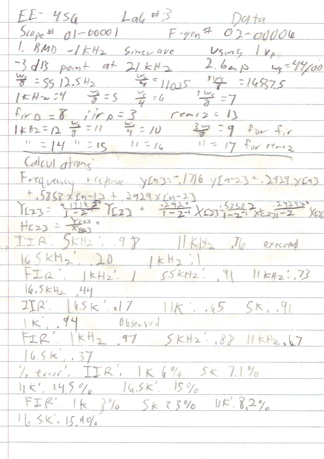
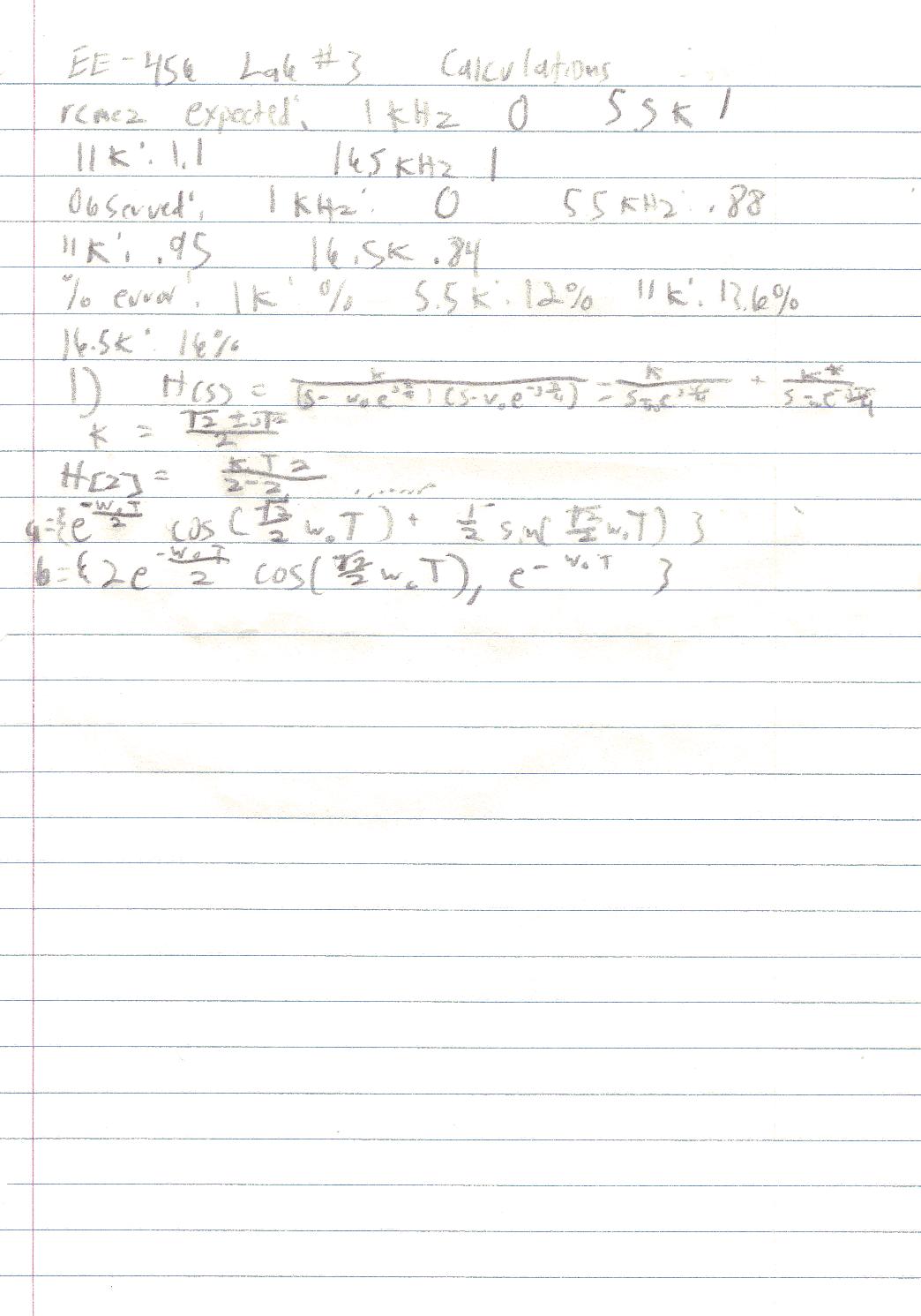
The objective of this lab is to investigate the effects of filter simulation using digital signal processing. Both IIR and FIR filters will be employed.
![]() Components Used
Components Used
1) Computer running Octave
2) Digital sampling board
3) Oscilloscope #01-00001
4) Function Generator #02-00006
![]() Procedures
Procedures
1) Using Octave, enter "iir(1,1)"
2) Enter command "ssrat(100000)"
3) Set the function generator
to generate a 1KHz sine wave with 2Vp
4) Observe the
output, it should mimic the input.
5) Vary the frequency up to 50KHz, and observe the output; it should continue to mimic the input.
6) Create an array a = [1.0, 0.0, .1716]
7) Create an array b = [.2929, .5858, .2929]
8) Using these coefficients, analytically solve and plot the transfer function for this filter.
9) Compute the expected frequency response at w = 0, ws/8, ws/4, and 3ws/8
10) Plot the resulting expected frequency response.
11) Use the command "iirp(b, a)" to plot the resulting frequency response.
12) Implement the filter using "iir(b, a)"
13) Set the function generator to 1KHz.
14) Observe the frequency response as the frequency is increased form 1KHz to 50KHz.
15) Using several points, estimate the frequency response.
16) Create an array b = [.5, .5].
17) Compute and plot the frequency response to this filter.
18) Use "firp(b)" to plot the frequency response.
19) Implement the filter using "fir(b)"
20) Repeat steps 13 to 15 to estimate the frequency response.
21) Create an array a = [0, 0, 1, 1, 1, 1, 0, 0] to simulate a band pass filter.
22) Enter command "f=0:7;"
23) Enter command "f=f/7;"
24) Using the remez command, and the newly generated f and a arrays, create an array b to simulate a 60 pole "brick wall" filter.
25) Plot this FIR filter.
26) Implement the filter.
27) Repeat steps 13 through 15 to estimate the frequency response.
![]() Lab
Data / Results
Lab
Data / Results
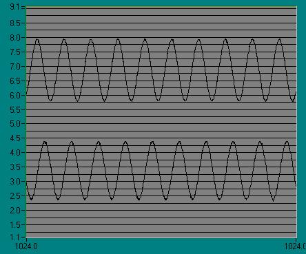
1) Diagram 1: 1KHz sine wave with no filtering:
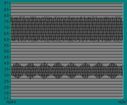
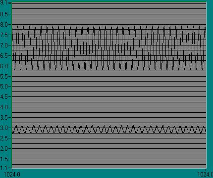
2) Diagram 2: 21KHz sine wave with no filtering:
3) Diagram
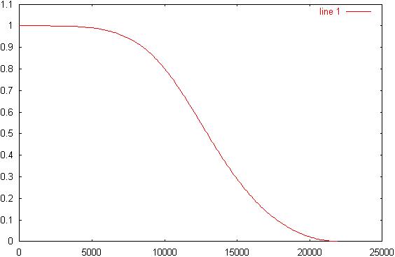
3: Expected frequency response for IIR filter:
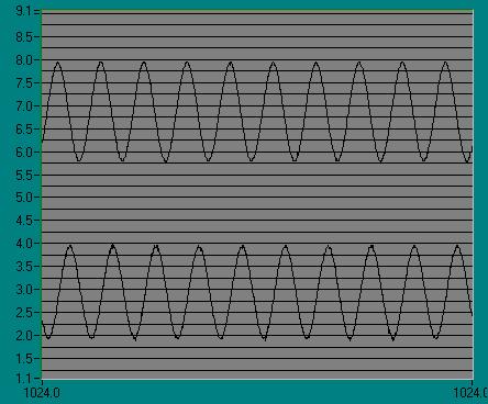
4) Diagram 4: 1KHz filtered sine wave:
5) Diagram
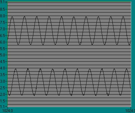
5: 5.5KHz filtered sine wave:
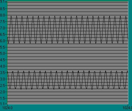
6) Diagram 6: 11KHz filtered sine wave:
7) Diagram 7: 16.5KHz filtered sine wave:
8) Table 1: Expected vs. observed frequency response for IIR filter:
|
Frequency: |
1KHz |
5.5KHz |
11KHz |
16.5KHz |
|---|---|---|---|---|
|
Expected: |
1.0 |
.98 |
.76 |
.20 |
|
Observed: |
.94 |
.91 |
.65 |
.17 |
|
%error: |
6.0% |
7.1% |
14.5% |
15.0% |
9) Table 2: Expected vs. observed frequency response for FIR filter:
|
Frequency: |
1KHz |
5.5KHz |
11KHz |
16.5KHz |
|---|---|---|---|---|
|
Expected: |
1.0 |
.91 |
.73 |
.44 |
|
Observed: |
.97 |
.88 |
.67 |
.37 |
|
%error: |
3.0% |
3.3% |
8.2% |
15.9% |
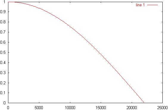
10) Diagram 8: Expected frequency response for FIR filter:
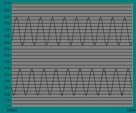
11) Diagram 9: 1KHz filtered sine wave:
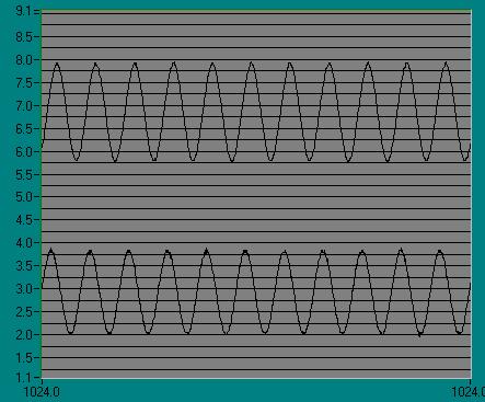
12) Diagram
10: 5.5KHz filtered sine wave:
13) Diagram
11: 11KHz filtered sine wave:
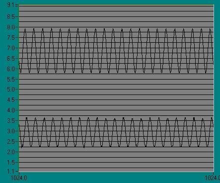
14) Diagram 12: 16.5KHz filtered sine wave:
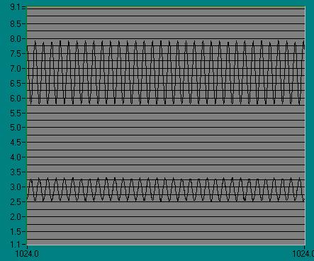
15) Diagram 13: Octave frequency plot for rimez filter:
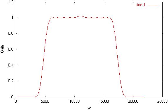
16) Diagram
14: 1KHz filtered sine wave:
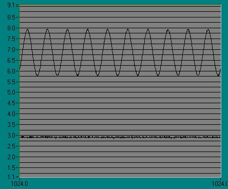
17) Diagram 15: 5.5KHz filtered sine wave:
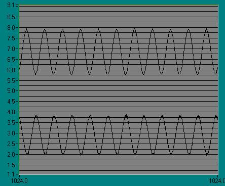
18) Diagram
16: 11KHz filtered sine wave:
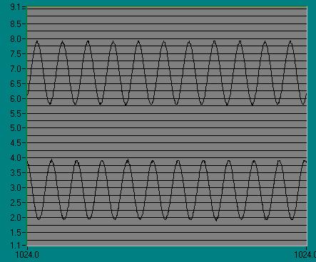
19) Diagram 17: 16.5KHz filtered sine wave:
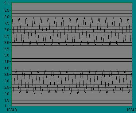
20) Table
3: Estimated frequency response for remez filter:
|
Frequency: |
1KHz |
5.5KHz |
11KHz |
16.5KHz |
|---|---|---|---|---|
|
Expected: |
0 |
1 |
1.1 |
1 |
|
Observed: |
0 |
.88 |
.95 |
.84 |
|
%error: |
0% |
12.0% |
13.6% |
16.0% |
![]() Answers to Lab Questions
Answers to Lab Questions
1) Q: What sequence of MatLab® commands would be required to implement a fourth order Butterworth low-pass filter whose cutoff frequency is ws/6?
A: 1) a = [e^((-ws/6) * T/2) * cos((2^(1/2) / 2) * (ws/6) * T) + (1/2) * sin((2^(1/2) / 2) * (ws / 6) * T), 0];
2) b = [2 * e^((-ws/6) * T / 2) * cos((2^(1/2) / 2 * (ws/6) * T), e^((ws/6) * T)];
3) iir(b,a)
2) Q: We wish to cascade two FIR filters with coefficients b1 and b2 using only one DSP. What sequence of MatLab® commands can accomplish this?
A: 1) b3 = conv(b1, b2);
2) fir(b3)
3) Q: What happens to the frequency response of an IIR filter as the poles approach the unit circle?
A: The cutoff frequency increases, and the system will begin to ring.
![]() Conclusions
Conclusions
This lab has demonstrated the effects of digital filtering on an signal. A majority of the error shown in Tables 1, 2, and 3 is the result of poor estimation of the expected gain and weight should not be as heavy on these values. Data in the lab was set up to compensate for a sampling rate of 44100. All data observed was based on this rate. Because a board with fixed sampling rate was used, the ssrat(100000) instruction was not used.
![]() Attachments
Attachments
