EE - 453 / E01 Fall 2003

Control I

Professor: Thomas

Submitted By:

Andrew Buettner

Partner:

Greg Kern

Lab #3: Study of Liquid Level Control System Using State Variable Method

Friday, December 12, 2003

Table Of Contents

1) Cover Page 1

2) Table of Contents 2

3) Objective 3

4) Components Used 3

5) Procedures 3

6) Lab Data / Results 3

1) Diagram 1 3

2) Table 1 4

3) Table 2 4

4) Table 3 4

5) Table 4 5

6) Table 5 5

7) Diagram 2 5

8) Diagram 3 6

9) Diagram 4 6

10) Diagram 5 7

11) Table 6 7

12) Table 7 7

13) Diagram 6 8

14) Diagram 7 8

15) Table 8 9

16) Table 9 9

7) Conclusions 9

8) Attachments 9

Objective

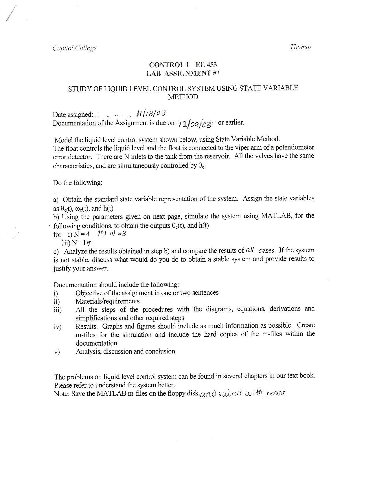
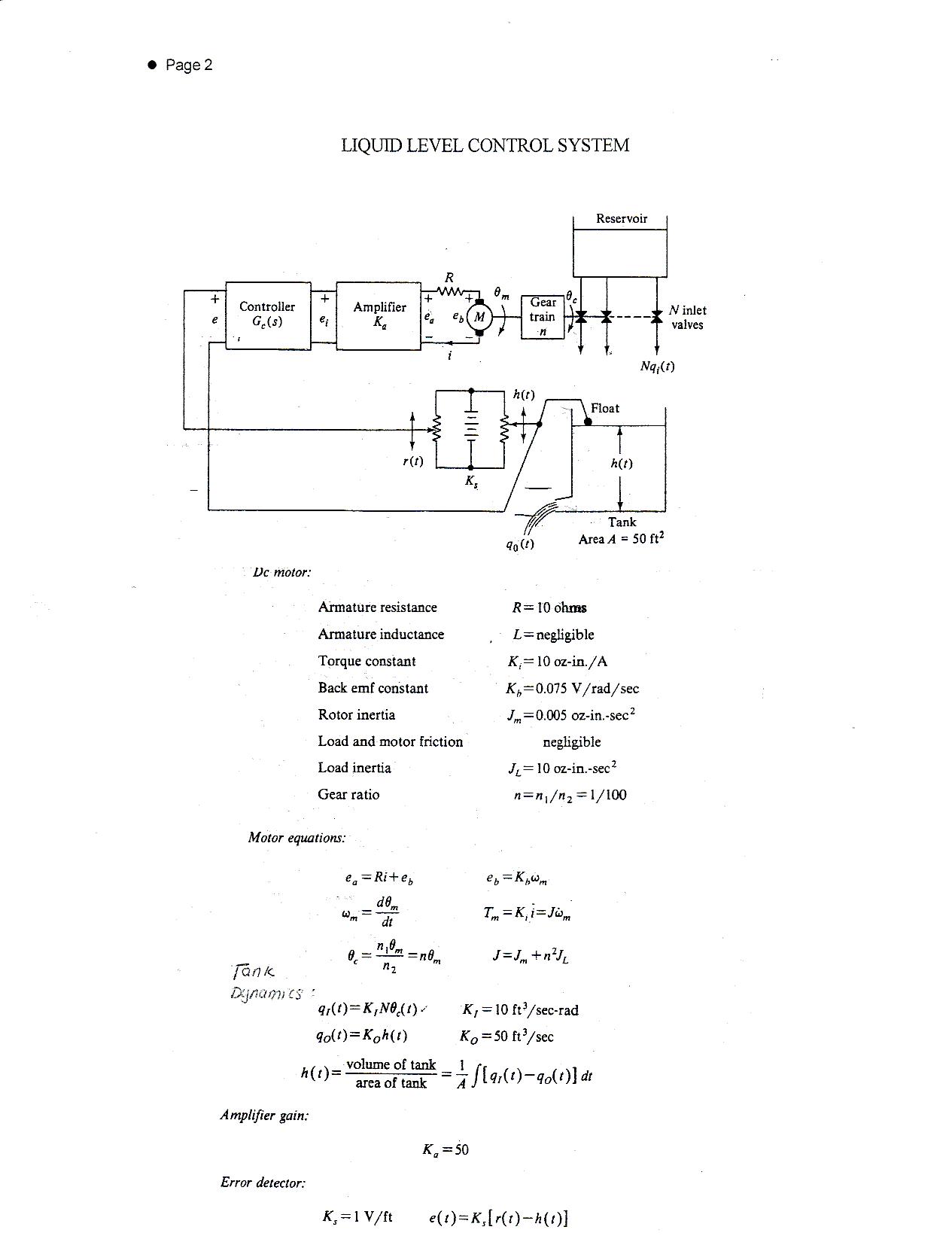
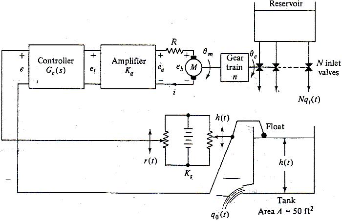
The objective of this lab is to model a water level control system and generate a state variable representation of it. The system is a tank with a drain pipe and several water inlets that are opened and closed by a motor driven by a differential amplifier. The water level is detected using a float that varies the voltage on a potentiometer. Using the data from the system, the number of inlet valves that are present to allow the system to be stable will be calculated. Also, the system will be modeled on MatLab® and the data will be used to determine weather or not the system is stable.

Components Used

1) PC with MatLab®, Octave®, or SciLab® installed.

Procedures

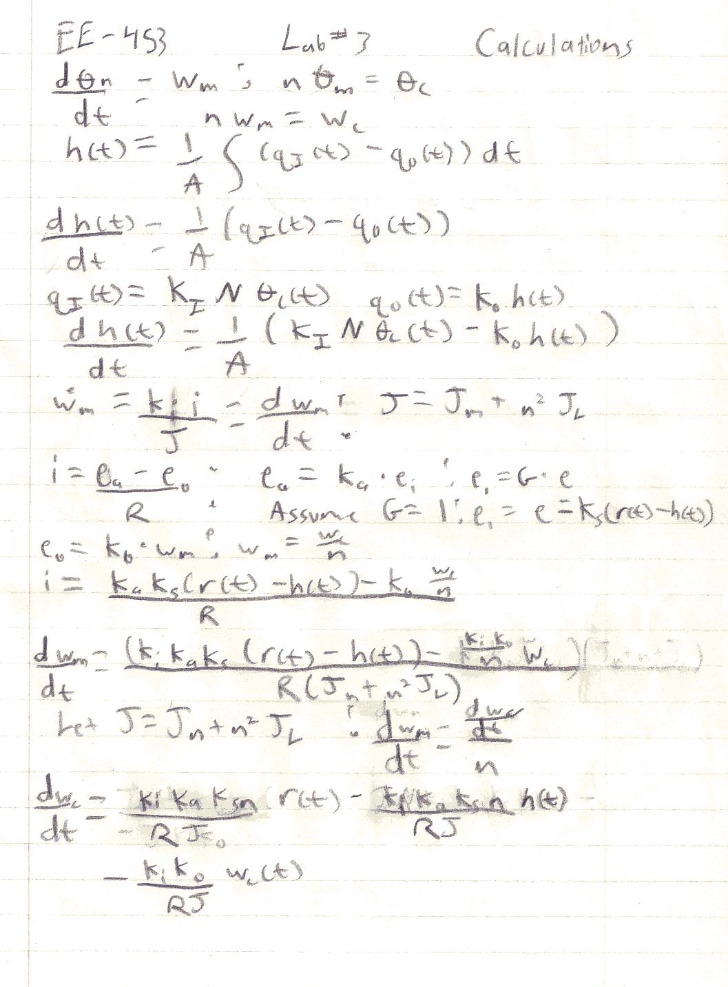
1) Obtain the state variable representation of the system using the following state variables: q_c(t), w_c(t), h(t).

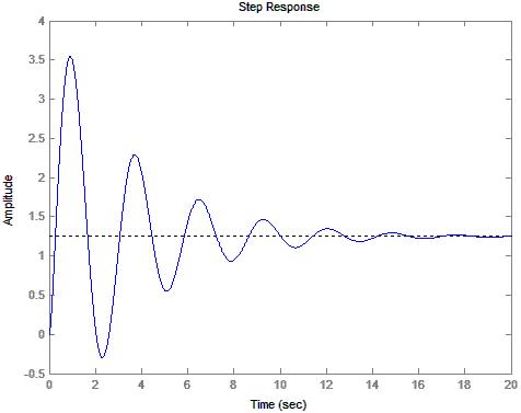
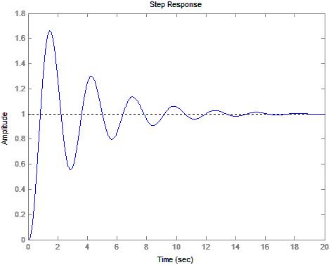
2) Using given values, simulate the system with N = 4 and obtain the outputs q_c(t) and h(t).

3) Determine if the system is stable.

4) Repeat steps 2 and 3 using N = 8.

5) Repeat steps 2 and 3 using N = 15.

Lab Data / Results

1) Diagram 1: Water Level System

2) Table 1: System Information

Parameter:

Value

Armature Resistance (R)

10W

Armature Inductance (L)

Negligible

Torque Constant (K_i)

10 oz*in/A

Back EMF Constant for Motor (K_b)

.075Vs/^r

Rotor Inertia (J_m)

.005oz*in*s²

Load and Motor Friction (F_m)

Negligible

Load Inertia (J_L)

10oz*in*s²

Gear Ratio (n₁:n₂) (n)

100:1

Valve Pour Constant (K_I)

10ft³/s*^r

Fill Rate (q_I(t))

K_I*N*q_c(t)

Drain Constant (K_O)

50ft³/s

Drain Rate (q_O(t))

K_O*h(t)

Amplifier Gain (K_a)

50

Detection Output (K_s)

1V/ft

Differential Amplifier Output (e(t))

K_s*(r(t) – h(t))

Total Torque on Motor (J)

J_m + n²*J_L

Parameter:	Value
Armature Resistance (R)	10W
Armature Inductance (L)	Negligible
Torque Constant (K_i)	10 ozin/A*
Back EMF Constant for Motor (K_b)	.075Vs/^r
Rotor Inertia (J_m)	.005ozins²
Load and Motor Friction (F_m)	Negligible
Load Inertia (J_L)	10ozins²
Gear Ratio (n₁:n₂) (n)	100:1
Valve Pour Constant (K_I)	10ft³/s^r*
Fill Rate (q_I(t))	K_INq_c(t)
Drain Constant (K_O)	50ft³/s
Drain Rate (q_O(t))	K_Oh(t)*
Amplifier Gain (K_a)	50
Detection Output (K_s)	1V/ft
Differential Amplifier Output (e(t))	K_s(r(t) – h(t))*
Total Torque on Motor (J)	J_m + n²J_L*

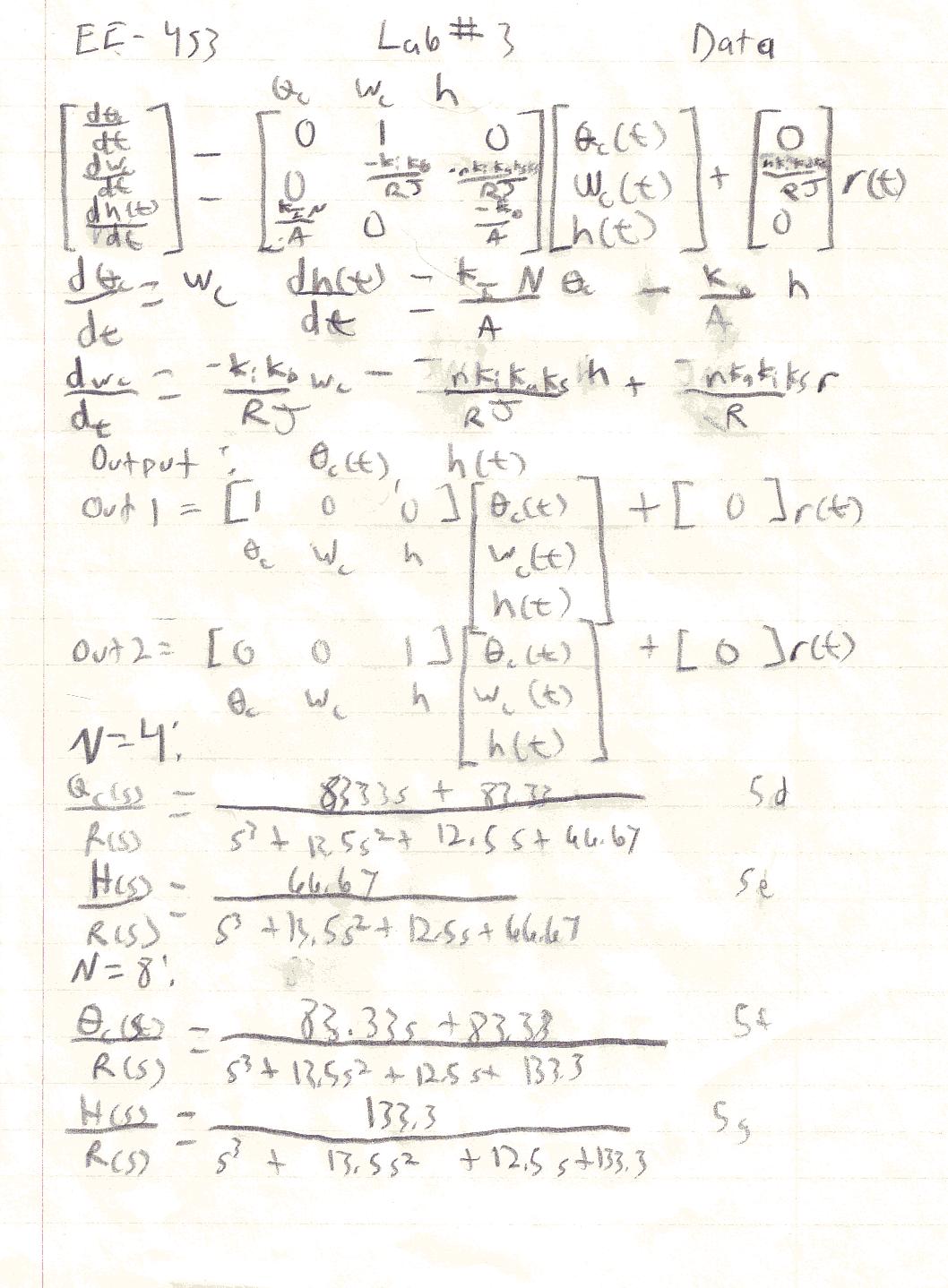
3) Table 2: Matrix Equation

dq_c(t)/dt

0

1

1

q_c(t)

0

dw_c(t)/dt

=

0

-(k_i*k_b)/(R*J)

-(n*k_i*k_a*k_s)/(R*J)

w_c(t)

+

(n*k_i*k_a*k_s)/

(R*J)

r(t)

dh(t)/dt

(k_I*N)/A

0

-k_O/A

h(t)

0

dq_c(t)/dt		0	1	1	q_c(t)		0
dw_c(t)/dt	=	0	-(k_ik_b)/(RJ)	-(nk_ik_ak_s)/(RJ)	w_c(t)	+	(nk_ik_ak_s)/ (RJ)	r(t)
dh(t)/dt		(k_IN)/A*	0	-k_O/A	h(t)		0

4) Table 3: Matrix Representation for q_c(t)

q_c(t)

=

1

0

0

q_c(t)

w_c(t)

+

0

r(t)

h(t)

5) Table 4: Matrix Representation for h(t)

q_c(t)

=

0

0

1

q_c(t)

w_c(t)

+

0

r(t)

h(t)

6) Table 5: Transfer Functions

N:

Response:

Transfer Function:

4

q_c(s)/R(s)

=

(83.33s + 83.33)/(s³ + 13.5s² + 12.5s + 66.67)

4

H(s)/R(s)

=

66.67/(s³ + 13.5s² + 12.5s + 66.67)

8

q_c(s)/R(s)

=

(83.33s + 83.33)/(s³ + 13.5s² + 12.5s + 133.3)

8

H(s)/R(s)

=

133.3/(s³ + 13.5s² + 12.5s + 133.3)

15

q_c(s)/R(s)

=

(83.33s + 83.33)/(s³ + 13.5s² + 12.5s + 250)

15

H(s)/R(s)

=

250/(s³ + 13.5s² + 12.5s + 250)

N:	Response:		Transfer Function:
4	q_c(s)/R(s)	=	(83.33s + 83.33)/(s³ + 13.5s² + 12.5s + 66.67)
4	H(s)/R(s)	=	66.67/(s³ + 13.5s² + 12.5s + 66.67)
8	q_c(s)/R(s)	=	(83.33s + 83.33)/(s³ + 13.5s² + 12.5s + 133.3)
8	H(s)/R(s)	=	133.3/(s³ + 13.5s² + 12.5s + 133.3)
15	q_c(s)/R(s)	=	(83.33s + 83.33)/(s³ + 13.5s² + 12.5s + 250)
15	H(s)/R(s)	=	250/(s³ + 13.5s² + 12.5s + 250)

7) Diagram 2: Output q_c(t) for N=4

8) Diagram 3: Output h(t) for N=4

9) Diagram 4: Output q_c(t) for N=8

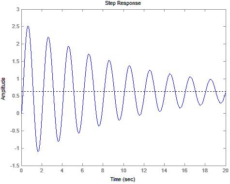
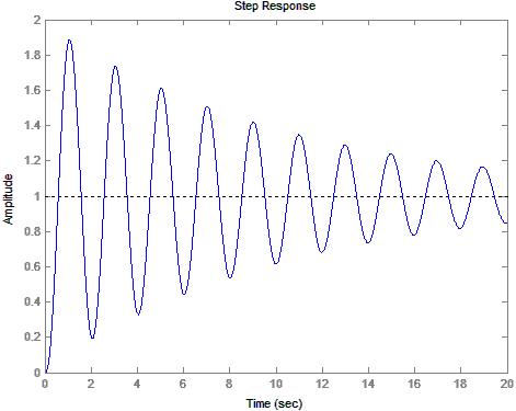
10) Diagram 5: Output h(t) for N=8

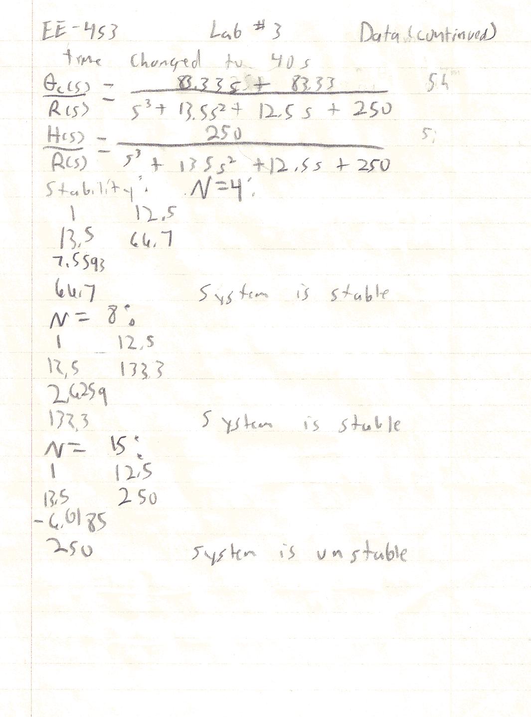
11) Table 6: Stability Calculations for N=4

s³

1

12.5

0

s²

13.5

66.7

0

s

7.5593

0

0

0

66.7

0

0

s³	1	12.5
s²	13.5	66.7
s	7.5593	0
0	66.7	0

12) Table 7: Stability Calculations for N=8

s³

1

12.5

0

s²

13.5

133.3

0

s

2.6259

0

0

0

133.3

0

0

s³	1	12.5
s²	13.5	133.3
s	2.6259	0
0	133.3	0

13) Diagram 6: Output q_c(t) for N=15

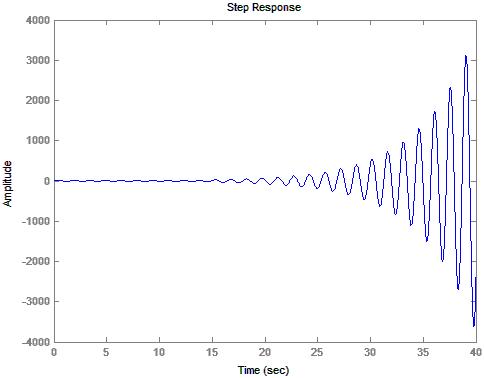
14) Diagram 7: Output h(t) for N=15

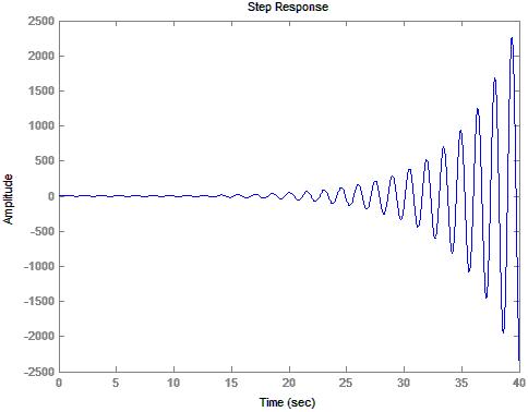
15) Table 8: Stability Calculations for N=15

s³

1

12.5

0

s²

13.5

250

0

s

-6.0185

0

0

0

250

0

0

s³	1	12.5
s²	13.5	250
s	-6.0185	0
0	250	0

16) Table 9: Stability Information

N

Predicted:

Observed:

4

Stable

Stable

8

Stable

Stable

16

Unstable

Unstable

N	Predicted:	Observed:
4	Stable	Stable
8	Stable	Stable
16	Unstable	Unstable

Conclusions

This lab has demonstrated how the MatLab® control toolbox can be used to take a state variable system and convert it to a transfer function in order to model a system. Both MatLab®, and the stability method discussed in class clearly show that the system loses stability as the number of inlet valves are added. I modeled the system observing only the first twenty seconds to determine weather or not the system would be stable. Twenty seconds was mostly an educated guess as to how long the system would take to stabilize. Upon observing the response at N=8 I changed the observation time to 40 seconds. This was also mostly an educated guess. The result, as observed is that the system is clearly unstable. Unfortunately, this lab does not take into account the fact that water can not flow “backwards” when the valves are shut off, nor can they open indefinitely. Additionally, the container can not hold negative water. These factors cause a significant deviation from what would normally be expected and therefore, the system would still most likely be stable with a much larger number of valves. However, the mathematics required to model the system would become significantly more difficult since the differential equations would have boundary conditions. The stable.m file is a straight forward implementation of the stability test that was discussed in class and should be able to run on MatLab® or any similar program with little to no modification.

Attachments

Original lab handout
Original lab data
Calculations
MatLab® log

>> water(4,1)

Transfer function:
83.33 s + 83.33
-------------------------------
s^3 + 13.5 s^2 + 12.5 s + 66.67


Transfer function:
66.67
-------------------------------
s^3 + 13.5 s^2 + 12.5 s + 66.67

>> water(8,1)

Transfer function:
83.33 s + 83.33
-------------------------------
s^3 + 13.5 s^2 + 12.5 s + 133.3


Transfer function:
133.3
-------------------------------
s^3 + 13.5 s^2 + 12.5 s + 133.3

>> water(15,1)

Transfer function:
83.33 s + 83.33
-----------------------------
s^3 + 13.5 s^2 + 12.5 s + 250


Transfer function:
250
-----------------------------
s^3 + 13.5 s^2 + 12.5 s + 250

>> den=[1 13.5 12.5 66.7];
>> stable(den)

a1 =

1.0000 12.5000 0 0


a2 =

13.5000 66.7000 0 0


b =

7.5593 0 0


b =

66.7000 0 0


b =

0 0 0

>> den=[1 13.5 12.5 133.3];
>> stable(den)

a1 =

1.0000 12.5000 0 0


a2 =

13.5000 133.3000 0 0


b =

2.6259 0 0


b =

133.3000 0 0


b =

0 0 0

>> den=[1 13.5 12.5 250];
>> stable(den)

a1 =

1.0000 12.5000 0 0


a2 =

13.5000 250.0000 0 0


b =

-6.0185 0 0


b =

250 0 0


b =

0 0 0