![]() Objective
Objective
The objective of this lab is is to simulate the modulation and demodulation of both FM and AM signals. The fft function will be used to verify the generated spectra to compare to a mathematically produced one.
![]() Components Used
Components Used
1) Computer With MatLab®, SciLab®, or Octave installed.
![]() Procedures
Procedures
1) Simulate an AM waveform with a carrier of 32Hz, a modulation of 3Hz and b of .75; use 256 samples.
2) Create a variable PHI that will be the fft of the original signal.
3) Use "plot(24:40, abs(PHI(25:41)))" to plot the spectrum.
4) Regenerate the original function and PHI with a modulated frequency of 2Hz, and a b of 2.
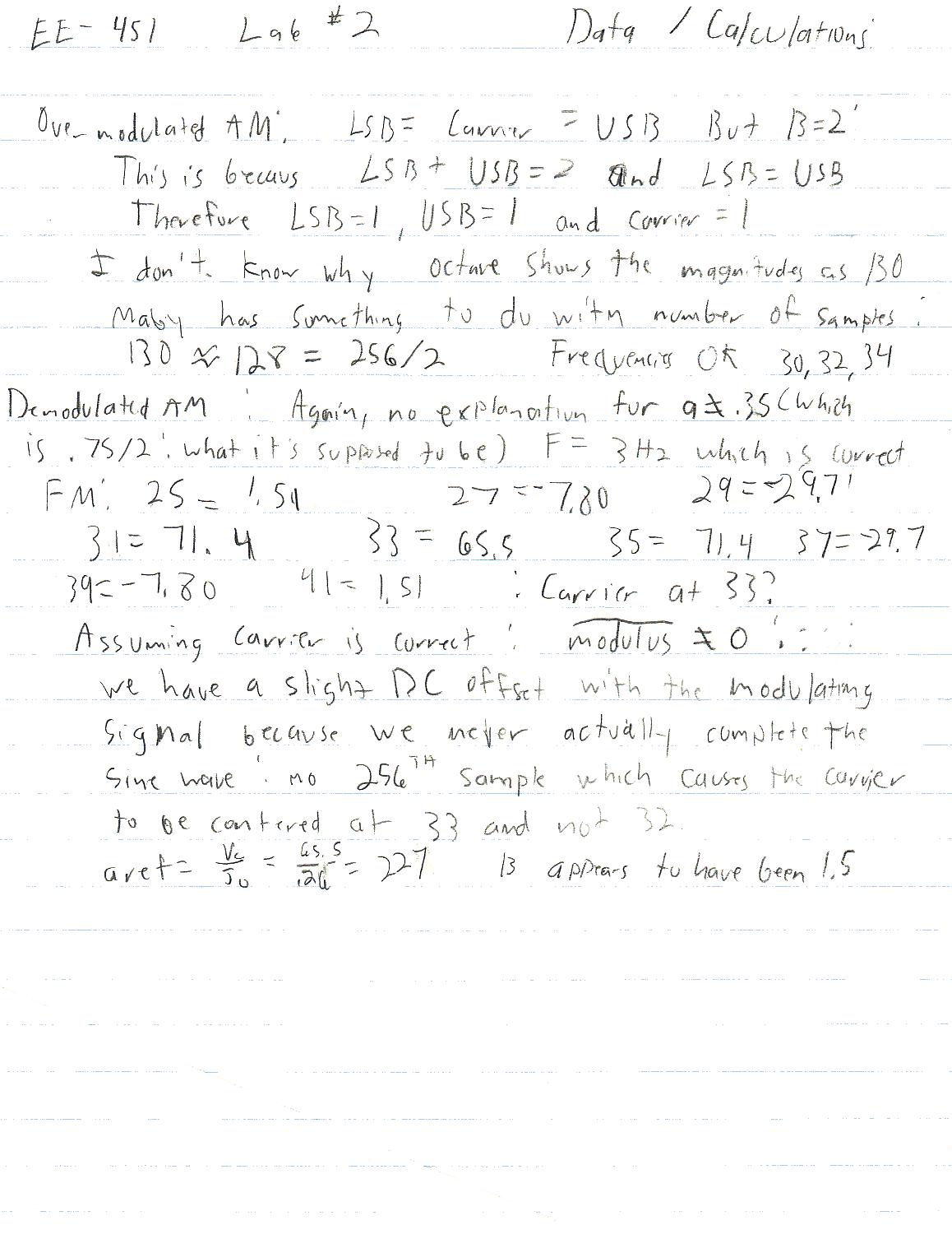
5) Explain the magnitudes and frequencies of the spectrum.
6) Reset the signal back to fm of 3Hz, and b of .75.
7) Simulate the demodulation of the signal by creating an additional function that contains only the positive values of the original function, and 0s otherwise.
8) Generate the spectrum of this new functions.
9) Generate a new function, H, that can be used to filter out all frequencies between 16Hz and 240Hz, and the DC component by:
a) H = zeros(1,256);
b) H(2:9) = ones(1,8);
c) f=0:126;
d) H(130:256) = H(128-f);
10) Multiply H and PR to create PRF.
11) Generate a time-domain signal, prf.
12) Justify the signal and it's spectrum.
13) Generate an FM signal with a carrier of 32Hz, a modulated frequency of 2Hz, and a mf of 3.
14) Plot the function and it's spectrum.
15) Justify the spectrum.
16) Create a transfer function that is a high pass filter to demodulate the FM signal:
a) f = 0:128;
b) HPF = ((f / 32). ^4) ./ (1 + (f / 32). ^4);
c) HPF = sqrt(HPF);
d) f=0:126;
e) HPF(130:256) = HPF(128-f);
17) Plot the HPF function.
18) Multiply the spectrum of the FM function with the transfer function to create the function D1.
19) Plot the new AM signal in the time domain.
20) Repeat steps 9 - 12 to demodulate the AM signal.
![]() Lab
Data / Results
Lab
Data / Results
1) Diagram 1: AM Waveform
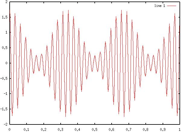
2) Diagram 2: AM Spectra
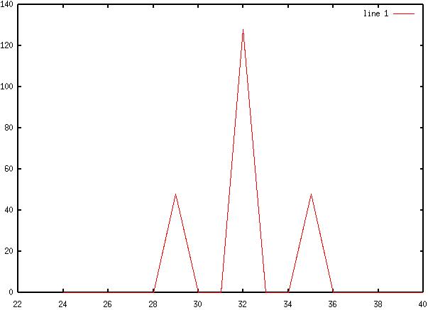
3) Diagram
3: Over-modulated AM Waveform
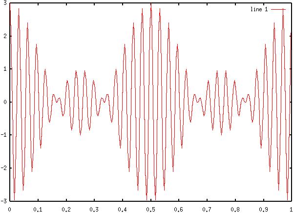
4) Diagram
4: Over-modulated AM Spectra
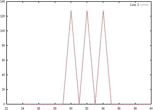
5) Diagram
5: Positive - Only AM waveform
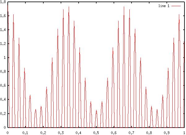
6) Diagram
6: Rectified AM Signal Spectra
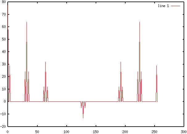
7) Diagram
7: Filtered, Rectified AM Signal Spectra
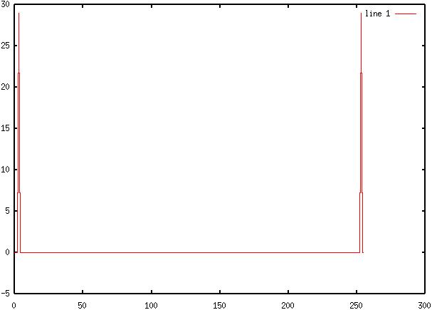
8) Diagram
8: Demodulated Time - Domain Signal
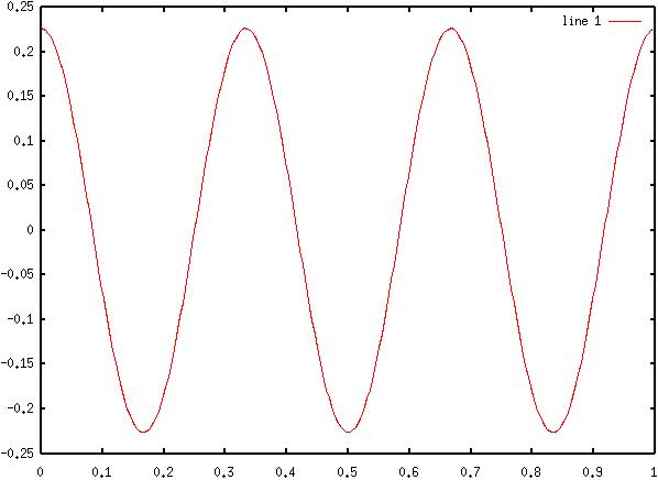
9) Diagram
9: FM Time - Domain Signal
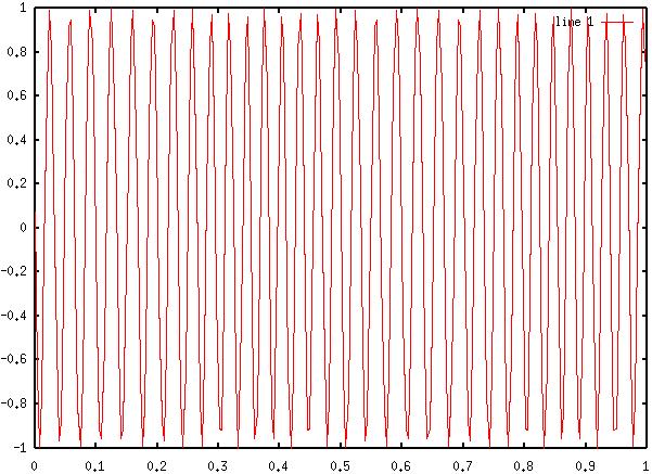
10) Diagram
10: FM Spectra
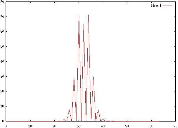
11) Diagram
11: High - Pass Filter Transfer Function
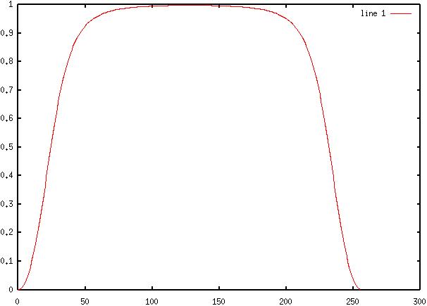
12) Diagram
12: Time - Domain Filtered AM - FM Signal
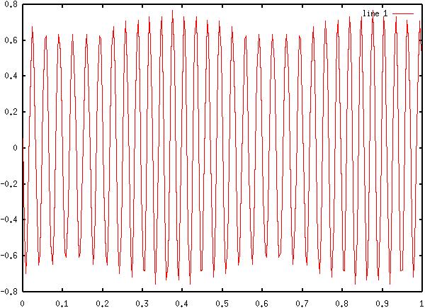
13) Diagram
13: Rectified Time - Domain AM - FM Signal
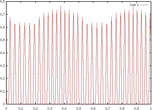
14) Diagram
14: Filtered AM - FM Signal Spectra
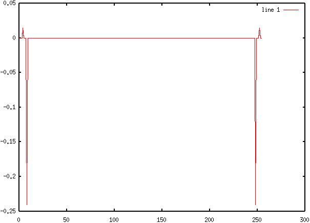
15) Diagram
15: Demodulated FM Signal
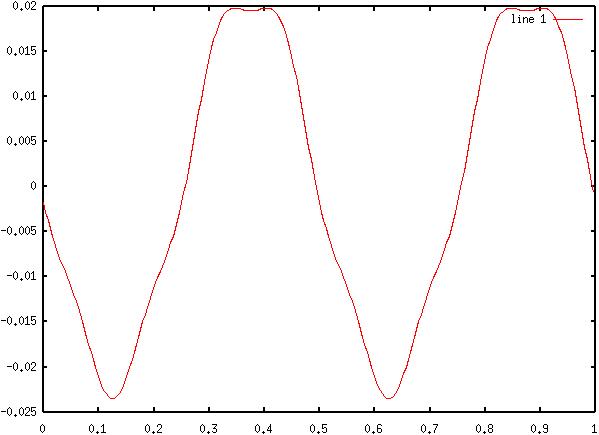
16) Table 1: FM Spectra Verification(b = 1.5!)
|
J |
Frequency |
Expected |
Observed |
%Error |
|---|---|---|---|---|
|
0 |
33Hz |
65.5 |
65.5 |
0.00% |
|
1 |
31Hz / 35Hz |
71.9 |
71.4 |
.695% |
|
2 |
29Hz / 37Hz |
29.5 |
29.7 |
.678% |
|
3 |
27Hz / 39Hz |
7.71 |
7.80 |
1.17% |
|
4 |
25Hz / 41Hz |
1.28 |
1.51 |
18.0% |
![]() Answers to Lab Questions
Answers to Lab Questions
1) Q: List two ways in which MatLab® can be used to compute the power of a signal.
A: 1) P=((x.*x').^2)./N (N is the number of samples in x)
2) P=((X.*X').^2)./(N/(2*pi)) (X = fft(x);)
2) Q: Write MatLab® code to generate and demodulate a DSB-SC signal: f=cos(wm*t)*cos(wc*t) - -sin(wm*t)*sin(wc*t) given that fc = 16Hz and fm = 2Hz.
A: 1) t=(0:255)/256;
2) phi=cos(2*pi*fc*t).*cos(2*pi*fm*t) + sin(2*pi*fc*t).*sin(2*pi*fm*t);
3) px=phi.*cos(2*pi*fc);
4) PX=fft(px);
5) H=zeros(1,256);
6) H(2:9)=ones(1,8);
7) f=0:126;
8) H(130:256)=H(128-f);
9) PXH = PX.*H;
10) pxh=ifft(PXH);
3) Q: Write MatLab® code to generate and demodulate a phase-modulated signal.
A: 1) t=(0:255)/256;
2) phi=cos(2*pi*fc*t-kp*cos(2*pi*fm*t));
3) PHI=fft(phi);
4) f=0:128;
5) HPF=((f/32).^4)./(1+(f/32).^4);
6) HPF=sqrt(HPF);
7) f=0:126;
8) HPF(130:256)=HPF(128-f);
9) PR=PHI.*HPF;
10) pr=ifft(pr);
11) pf = pr;
12) for i = 1:255, if pf(i) < 0
13) pf(i) = 0;
14) end,
15) end
16) PF=fft(pf);
17) H=zeros(1,256);
18) H(2:9)=ones(1,8);
19) f=0:126;
20) H(130:256)=H(128-f);
21) PRH=PR.*H;
22) prh=ifft(PRH);
![]() Conclusions
Conclusions
This lab has demonstrated various methods of simulating the demodulation a modulated signal. Both AM and FM were demodulated in this lab, as well as methods for demodulating SSB-SC and phase modulation. These four modulation - demodulation techniques form the basis of almost every means for wireless communication today. Interestingly, for the FM modulation, since a the modulating sine wave was one sample short of a complete wave, the wave had a positive DC offset, which was interpreted by the simulation as a higher carrier frequency. Although the log will reveal that the carrier frequency was set to 32Hz, the observed carrier was 33Hz. Please consult the hand written notes in the attachments section for further details, along with other notes made while observing the simulations. The b of the FM signal was observed to be 1.5. This is even though the equation entered was "2*b*cos(wm*t)." I have no explanation for why this happened. For a follow up, I tried a higher frequency example of the FM using x=cos((wc+wm*b*cos(wm*t)).*t). I had no success at reproducing a correct FM spectra. I also attempted increasing the number of samples taken form 256 to 1024. This did not improve the situation either. For some reason, I can not simulate a linear relationship between carrier frequency and modulation voltage, which is the driving force in any VCO, and VCOs are commonly used as cheap FM signal generators. Even reactance based modulators use this principle. The only FM modulator that does not use this principle is the NBFM modulator made by phase shifting the carrier with respect to the modulation. I can not remember the term given to this modulator, I do remember that if the signals are added, it is FM and if they are subtracted it is PM. I do not believe that user error can be totally eliminated in this situation as I have little experience with MatLab® based applications. On another note, this lab used Octave exclusively for simulation. I believe that Octave has the better interface, and will therefore use it more often.
![]() Attachments
Attachments
